Computational Efficiency: ttm vs rTensor
We compare the computational efficiency of the ttm
function from the tensory package with the equivalent
function in the rTensor package. This benchmark
demonstrates the performance benefits of using tensory for
tensor-times-matrix multiplication.
set.seed(123)

# Create a random 3-mode tensor and a matrix
X <- array(runif(30*40*50), dim = c(30, 40, 50))
mat <- matrix(runif(20*40), nrow = 20, ncol = 40)

library(bench)

# Prepare rTensor object
X_rTensor <- rTensor::as.tensor(X)
X <- tensory::Tensor$new(X)

# Benchmark ttm in tensory vs rTensor
bm <- bench::mark(
  tensory = tensory::ttm(X, mat, mode = 2)$data,
  rTensor = rTensor::ttm(X_rTensor, mat, m = 2)@data,
  min_iterations = 50,
  check = FALSE
)
bm
#> # A tibble: 2 × 6
#>   expression      min   median `itr/sec` mem_alloc `gc/sec`
#>   <bch:expr> <bch:tm> <bch:tm>     <dbl> <bch:byt>    <dbl>
#> 1 tensory      1.74ms   1.84ms      514.   511.1KB     4.11
#> 2 rTensor      1.76ms   1.82ms      538.     1.2MB    15.4


# Visualization
library(ggplot2)
library(dplyr)
library(tidyr)
autoplot(bm, type = "violin")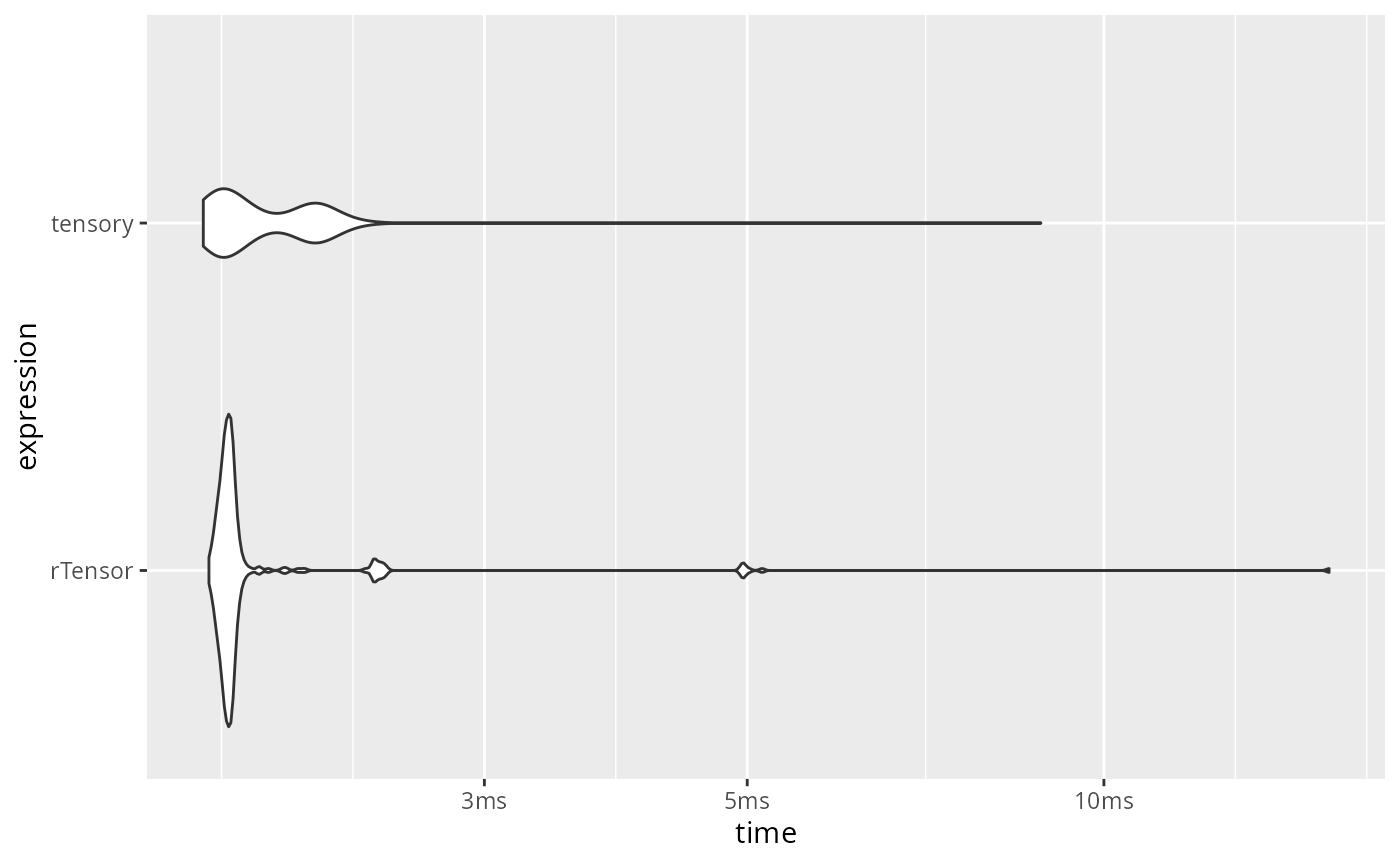
bm %>%
  unnest(c(time, gc)) %>%
  filter(gc == "none") %>%
  mutate(expression = as.character(expression)) %>%
  ggplot(aes(x = mem_alloc, y = time, color = expression)) +
  geom_point() +
  scale_color_bench_expr(scales::brewer_pal(type = "qual", palette = 3))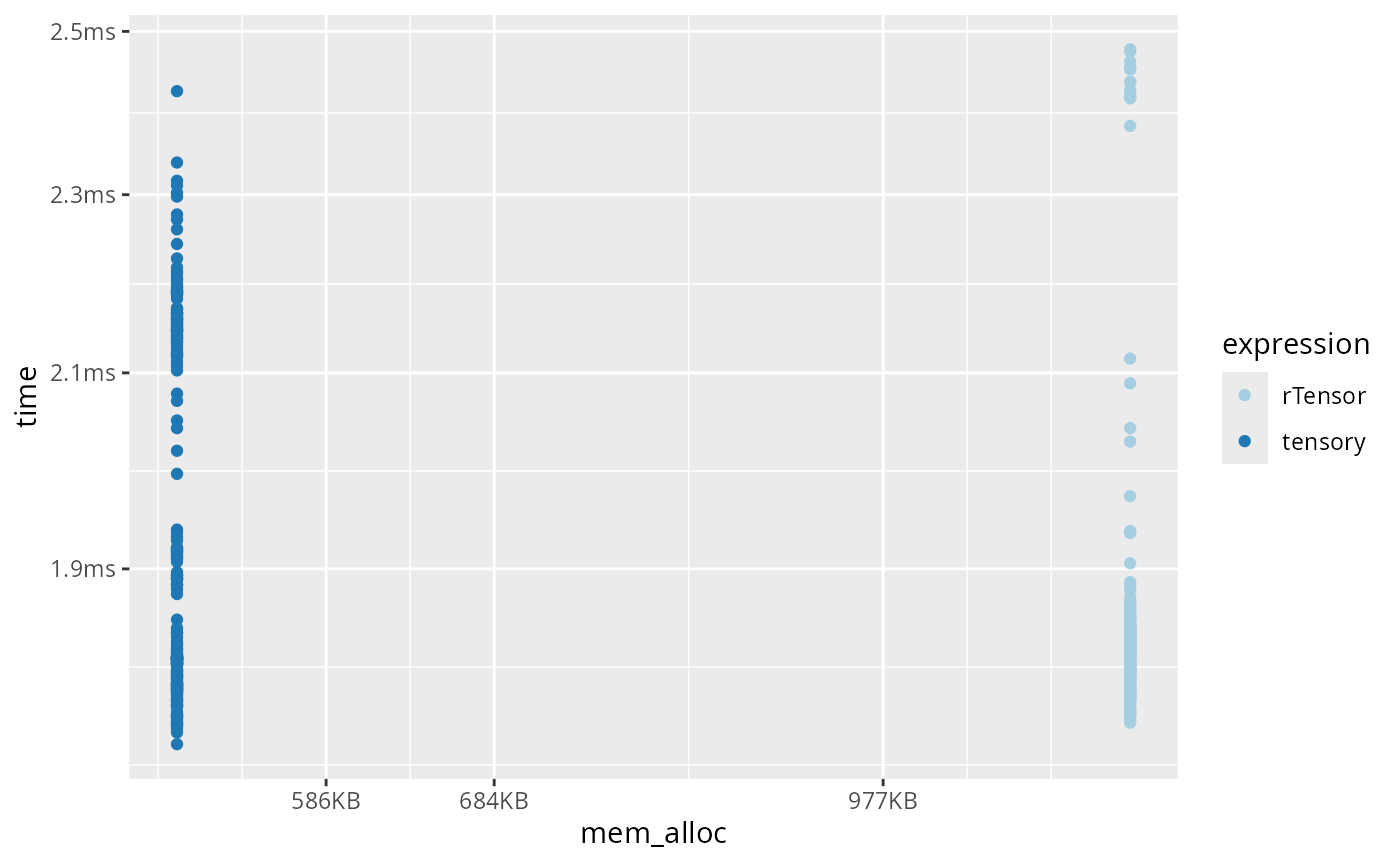
set.seed(123)

# Create a random 3-mode tensor and a matrix
X <- array(runif(10*100*50), dim = c(10, 100, 50))
mat <- matrix(runif(100*100), nrow = 100, ncol = 100)

library(bench)

# Prepare rTensor object
X_rTensor <- rTensor::as.tensor(X)
X <- tensory::Tensor$new(X)

# Benchmark ttm in tensory vs rTensor
bm <- bench::mark(
  tensory = tensory::ttm(X, mat, mode = 2)$data,
  rTensor = rTensor::ttm(X_rTensor, mat, m = 2)@data,
  iterations = 50,
  check = FALSE
)
bm
#> # A tibble: 2 × 6
#>   expression      min   median `itr/sec` mem_alloc `gc/sec`
#>   <bch:expr> <bch:tm> <bch:tm>     <dbl> <bch:byt>    <dbl>
#> 1 tensory      4.32ms   4.88ms      204.  781.67KB     4.16
#> 2 rTensor      4.32ms   5.19ms      197.    1.53MB     8.22

# Visualization
library(ggplot2)
autoplot(bm, type = "violin")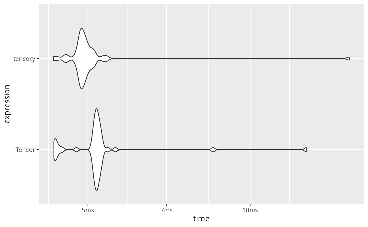
Multiple Matrix Multiplications Benchmark
Here we benchmark the performance of multiple matrix multiplications, which is a common operation in tensor decomposition algorithms and multilinear algebra.
set.seed(456)

# Create a 4-mode tensor and matrices for each mode
X3 <- array(runif(50*40*30*20), dim = c(50, 40, 30, 20))
matrices3 <- list(
  matrix(runif(6*50), nrow = 6, ncol = 50),  # mode 1
  matrix(runif(4*40), nrow = 4, ncol = 40),  # mode 2
  matrix(runif(3*30), nrow = 3, ncol = 30),  # mode 3
  matrix(runif(2*20), nrow = 2, ncol = 20)   # mode 4
)

library(bench)

# Prepare rTensor object
X3_rTensor <- rTensor::as.tensor(X3)
X3_tensor <- tensory::Tensor$new(X3)

# Define function for multiple rTensor ttm operations
multiple_ttm_rTensor <- function(tensor, mat_list) {
  result <- tensor
  for (i in seq_along(mat_list)) {
    result <- rTensor::ttm(result, mat_list[[i]], m = i)
  }
  return(result)
}

# Benchmark multiple ttm operations
bm_multiple <- bench::mark(
  tensory = tensory::ttm(X3_tensor, matrices3, mode = c(1, 2, 3, 4))$data,
  rTensor = multiple_ttm_rTensor(X3_rTensor, matrices3)@data,
  iterations = 50,
  check = FALSE
)
bm_multiple
#> # A tibble: 2 × 6
#>   expression      min   median `itr/sec` mem_alloc `gc/sec`
#>   <bch:expr> <bch:tm> <bch:tm>     <dbl> <bch:byt>    <dbl>
#> 1 tensory      12.3ms   14.3ms      70.5    1.08MB     4.50
#> 2 rTensor        13ms   13.3ms      73.7   14.07MB    73.7

# Visualization
library(ggplot2)
autoplot(bm_multiple, type = "violin")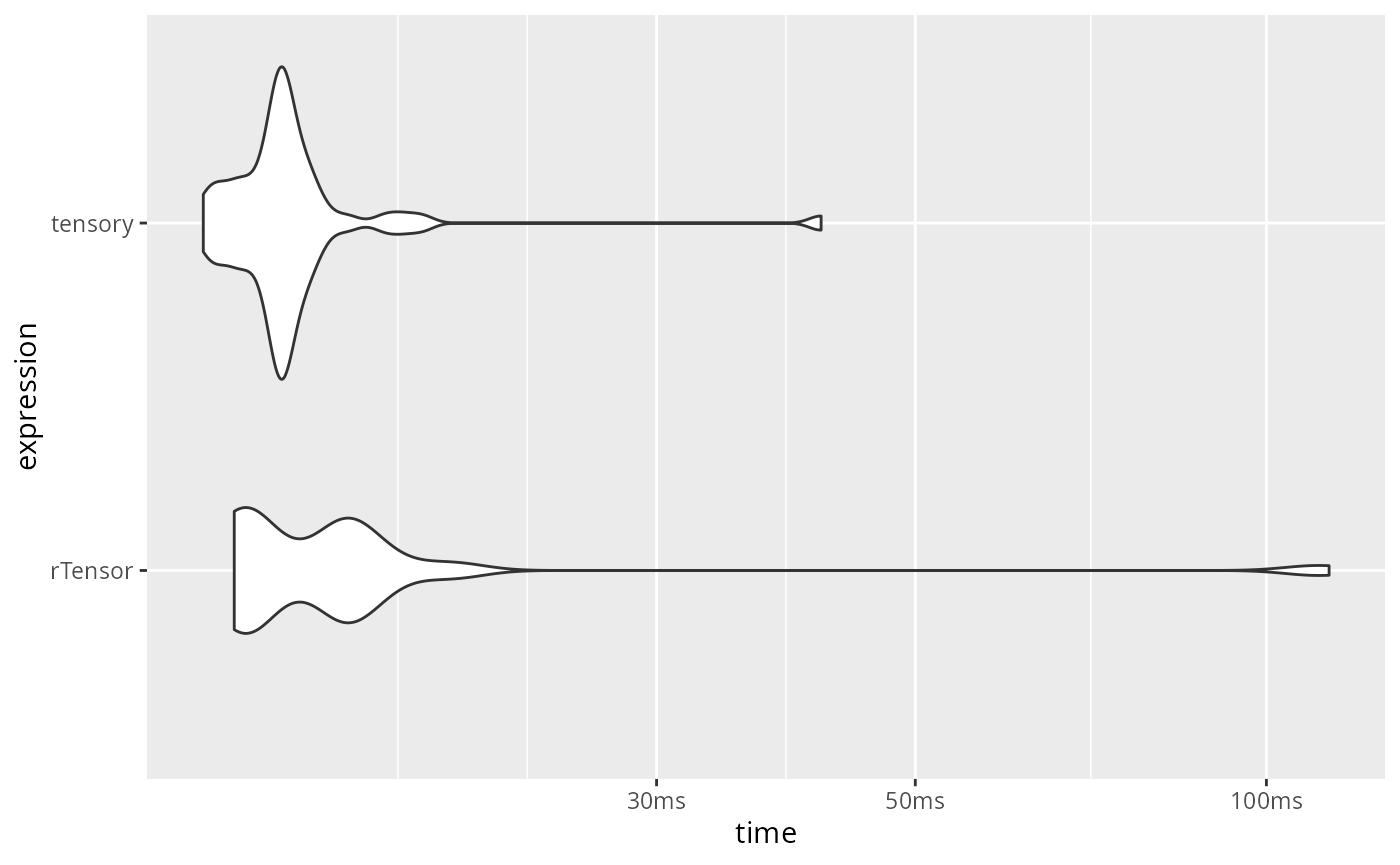
set.seed(456)

# Create a 4-mode tensor and matrices for each mode
X <- array(runif(4^6), dim = rep(4,6))
a <- matrix(runif(4*4), nrow = 4, ncol = 4)
matrices <- lapply(1:6,function(xx) a)

library(bench)

# Prepare rTensor object
X_rTensor <- rTensor::as.tensor(X)
X <- tensory::Tensor$new(X)

# Define function for multiple rTensor ttm operations
multiple_ttm_rTensor <- function(tensor, mat_list) {
  result <- tensor
  for (i in seq_along(mat_list)) {
    result <- rTensor::ttm(result, mat_list[[i]], m = i)
  }
  return(result)
}

# Benchmark multiple ttm operations
bm_multiple <- bench::mark(
  tensory = tensory::ttm(X, matrices, mode = 1:6)$data,
  rTensor = multiple_ttm_rTensor(X_rTensor, matrices)@data,
  iterations = 10,
  check = FALSE
)
bm_multiple
#> # A tibble: 2 × 6
#>   expression      min   median `itr/sec` mem_alloc `gc/sec`
#>   <bch:expr> <bch:tm> <bch:tm>     <dbl> <bch:byt>    <dbl>
#> 1 tensory    954.77µs 986.36µs     1016.     225KB        0
#> 2 rTensor      2.01ms   2.05ms      486.     773KB        0

# Visualization
library(ggplot2)
autoplot(bm_multiple, type = "violin")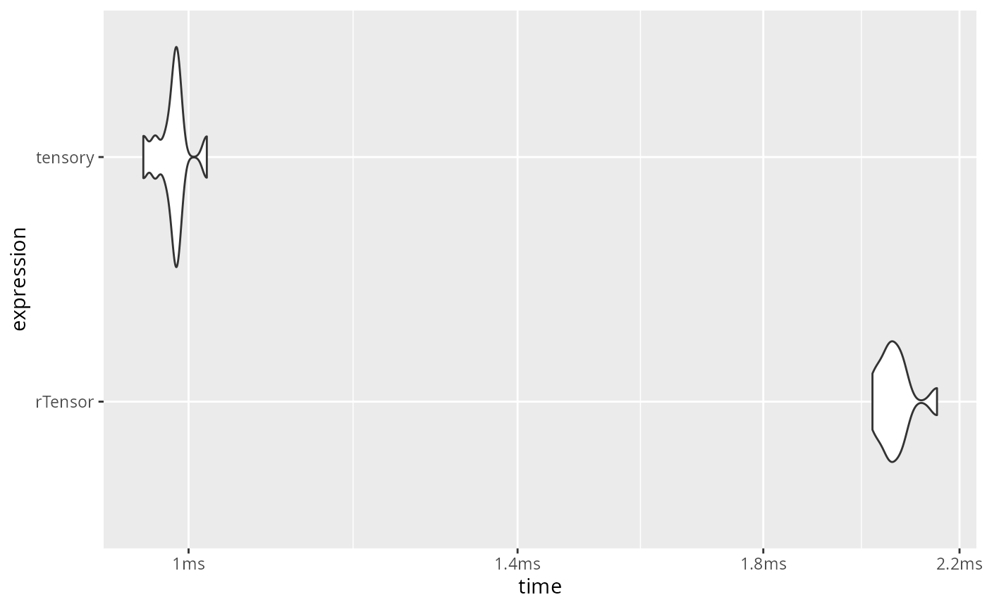
Memory Efficiency Comparison
Let’s also compare memory usage during these operations:
set.seed(789)

# Create a tensor and matrix for memory comparison
X <- array(runif(30*25*20), dim = c(30, 25, 20))
mat <- matrix(runif(35*25), nrow = 35, ncol = 25)

library(bench)

# Prepare rTensor object
X_rTensor <- rTensor::as.tensor(X)
X <- tensory::Tensor$new(X)

# Memory benchmark
bm_memory <- bench::mark(
  tensory = tensory::ttm(X, mat, mode = 2)$data,
  rTensor = rTensor::ttm(X_rTensor, mat, m = 2)@data,
  iterations = 20,
  check = FALSE
)
bm_memory
#> # A tibble: 2 × 6
#>   expression      min   median `itr/sec` mem_alloc `gc/sec`
#>   <bch:expr> <bch:tm> <bch:tm>     <dbl> <bch:byt>    <dbl>
#> 1 tensory       700µs    744µs     1357.     329KB        0
#> 2 rTensor       798µs    831µs     1201.     610KB        0

# Visualization
library(ggplot2)
autoplot(bm_memory, type = "violin")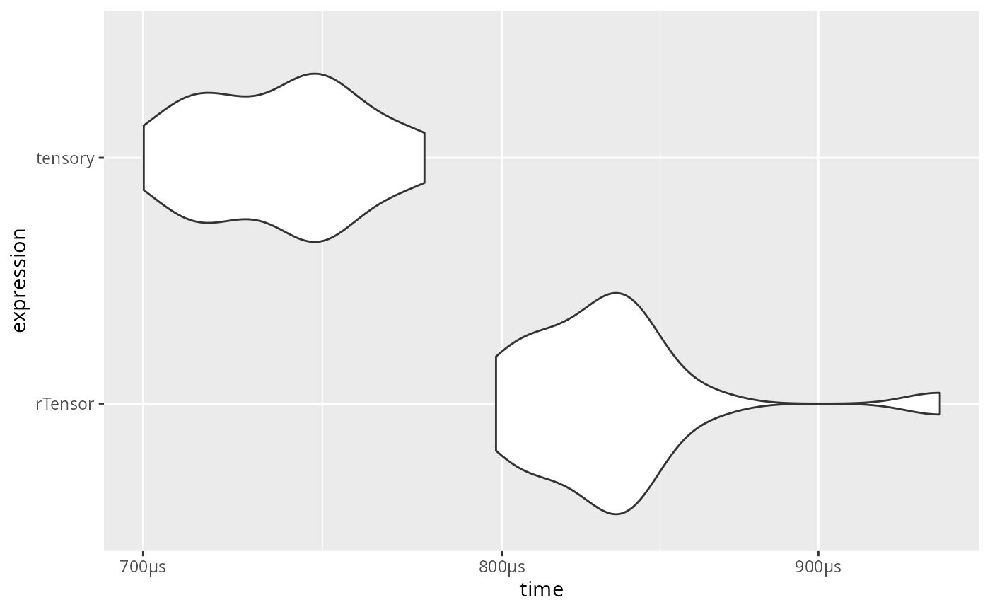
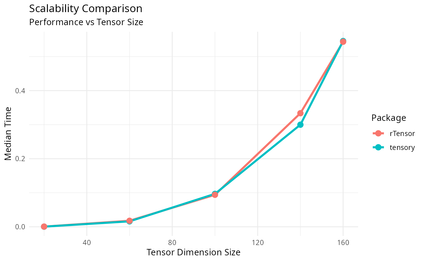
Scalability Analysis
Finally, let’s analyze how performance scales with tensor size:
set.seed(101112)

# Test different tensor sizes
sizes <- c(20, 60, 100, 140, 160)
scalability_results <- data.frame()

library(bench)

for (size in sizes) {
  # Create tensor of varying size
  X <- array(runif(size^3), dim = c(size, size, size))
  mat <- matrix(runif((size) * size), nrow = size, ncol = size)

  # Prepare rTensor object
  X_rTensor <- rTensor::as.tensor(X)
  X <- tensory::Tensor$new(X)

  # Benchmark
  bm_scale <- bench::mark(
    tensory = tensory::ttm(X, mat, mode = 2)$data,
    rTensor = rTensor::ttm(X_rTensor, mat, m = 2)@data,
    iterations = 20,
    check = FALSE
  )

  # Store results
  temp_results <- data.frame(
    size = size,
    package = as.character(bm_scale$expression),
    median_time = as.numeric(bm_scale$median),
    memory = as.numeric(bm_scale$mem_alloc)
  )

  scalability_results <- rbind(scalability_results, temp_results)
}

# Visualization
library(ggplot2)
ggplot(scalability_results, aes(x = size, y = median_time, color = package)) +
  geom_line(size = 1.2) +
  geom_point(size = 3) +
  #scale_y_log10() +
  labs(title = "Scalability Comparison",
       subtitle = "Performance vs Tensor Size",
       x = "Tensor Dimension Size",
       y = "Median Time",
       color = "Package") +
  theme_minimal()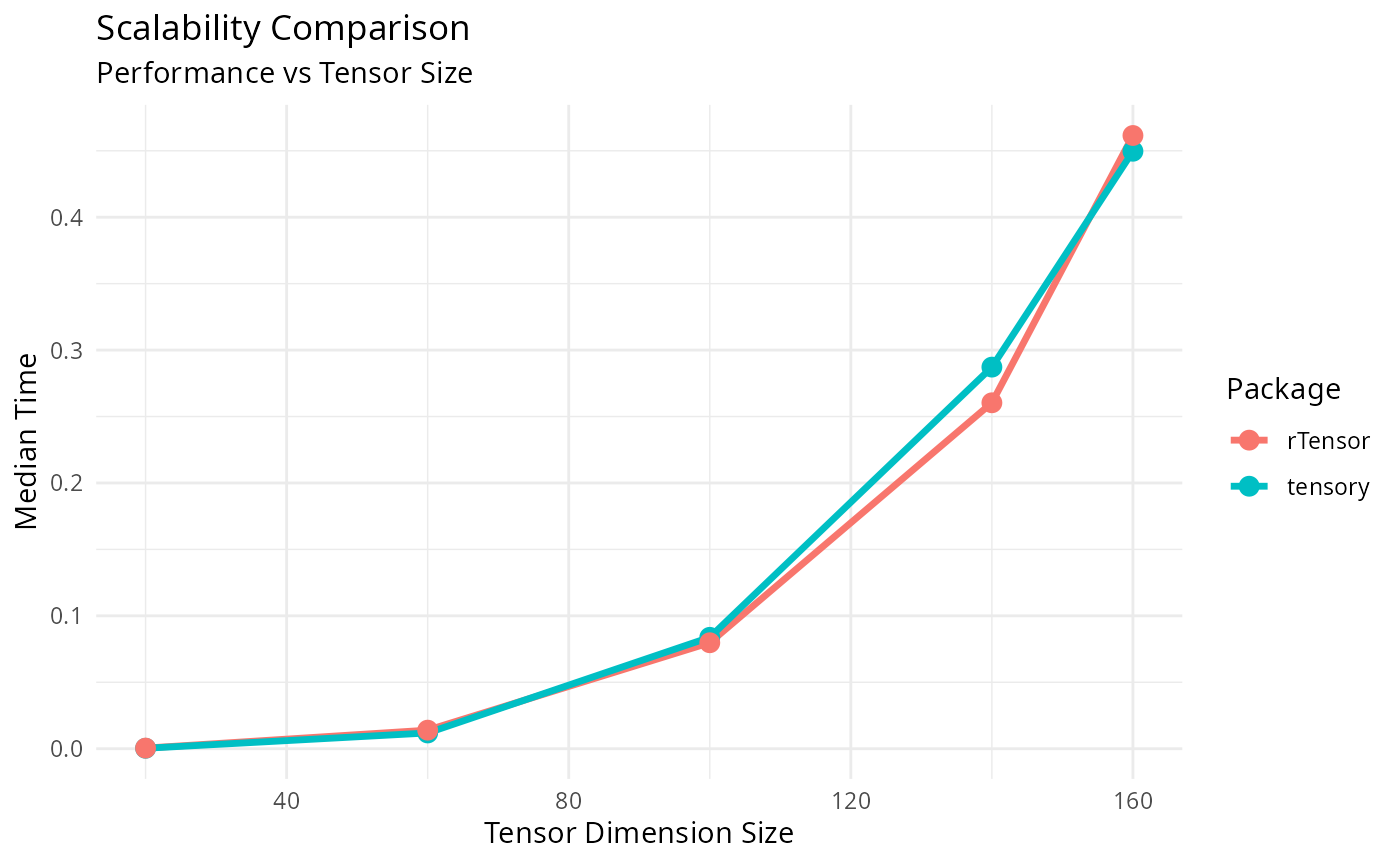
set.seed(101112)

# Test different tensor sizes
sizes <- c(20, 60, 100, 140, 160)
scalability_results <- data.frame()

library(bench)

for (size in sizes) {
  # Create tensor of varying size
  X <- array(runif(size*size*size), dim = c(size, size, size))
  mat <- matrix(runif((size+10) * size), nrow = size+10, ncol = size)

  # Prepare rTensor object
  X_rTensor <- rTensor::as.tensor(X)
  X <- tensory::Tensor$new(X)

  # Benchmark
  bm_scale <- bench::mark(
    tensory = tensory::ttm(X, mat, mode = 3)$data,
    rTensor = rTensor::ttm(X_rTensor, mat, m = 3)@data,
    iterations = 10,
    check = FALSE
  )

  # Store results
  temp_results <- data.frame(
    size = size,
    package = as.character(bm_scale$expression),
    median_time = as.numeric(bm_scale$median),
    mean_time = as.numeric(bm_scale$total_time/bm_scale$n_itr),
    memory = as.numeric(bm_scale$mem_alloc)
  )

  scalability_results <- rbind(scalability_results, temp_results)
}

# Visualization
library(ggplot2)
ggplot(scalability_results, aes(x = size, y = mean_time, color = package)) +
  geom_line(size = 1.2) +
  geom_point(size = 3) +
  #scale_y_log10() +
  labs(title = "Scalability Comparison",
       subtitle = "Performance vs Tensor Size",
       x = "Tensor Dimension Size",
       y = "Median Time",
       color = "Package") +
  theme_minimal()