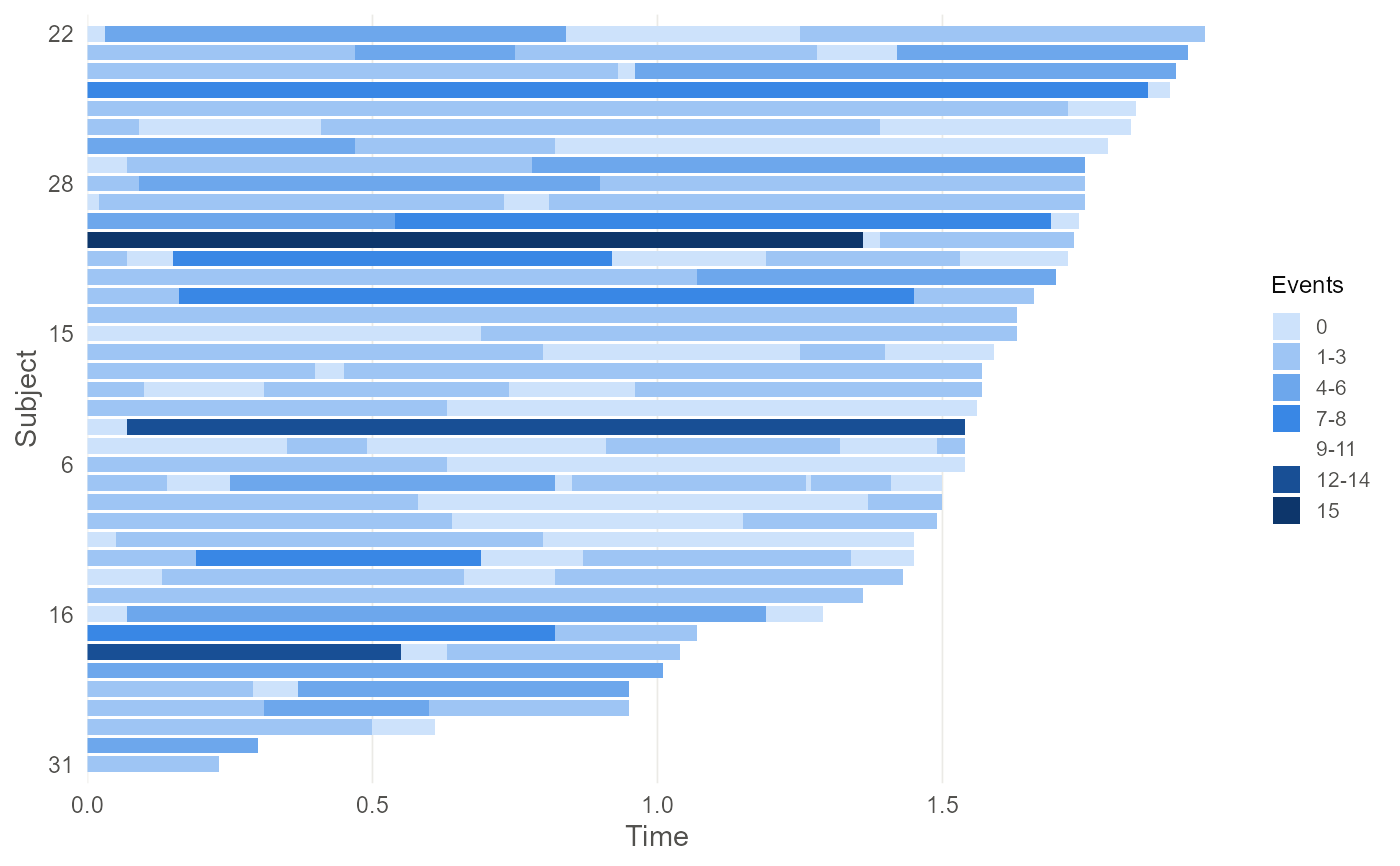
Draws the observation pattern as tiles: one row per subject, one tile per examination interval spanning the time it covers, shaded by the number of events recorded in it.
Arguments
- object, x
A
pcd()object.- order_by
How to order subjects up the vertical axis.
"followup"sorts by the time of the last examination, which makes the censoring pattern legible;"events"sorts by the total number of events;"none"keeps the order of the identifiers.- max_subjects
Draw at most this many subjects, taken as an evenly spaced sample so the picture stays readable for large studies. A message reports how many were shown.
- palette
Fill colours, lightest first. The default is a single-hue sequential ramp, which is where a magnitude belongs.
- ...
Ignored.
Value
A ggplot2::ggplot() object, so it can be titled, faceted or
themed like any other. autoplot() returns it; plot() draws it and
returns it invisibly, so it can be used for its side effect like any
other plot() method.
Details
The tile is the unit of observation. A panel count is attributed to the interval \((T_{i,j-1}, T_{ij}]\) rather than to an instant, so drawing the intervals rather than points at the examination times is what the data actually says: a wide pale tile and a narrow dark one can carry the same count while meaning very different things about the rate.
Two features decide how an analysis will go and both are visible here. Whether examination times line up across subjects sets the size of the pooled grid and so the cost of fitting the rate model; and how ragged the right hand edge is shows how much of the tail of the baseline rests on a handful of subjects.
See also
autoplot.pcdfit() for the fitted baseline function.