Where pcdreg fits among R packages for panel count data

library(pcdreg)

This article describes the settings in which pcdreg and the available alternatives apply.

The landscape

Three classes of R package address recurrent event data. They are not interchangeable.

Exactly observed event times. If you know when each event happened, reReg, survival, and the recurrent-event literature apply. The discussion below concerns panel count data, where only the number of events between visits is known.

spef, by Chiou, Wang and Yan, is the established R package for panel count data. It offers a wide range of estimators through one function, panelReg(formula, data, method = ...). These include augmented estimating equations for an informative observation process (AEE, AEEX), maximum pseudolikelihood and monotone spline likelihood methods (MPL, MPLs, MLs), the Sun–Wei and Hu–Sun–Wei estimating equations, and an accelerated mean model. Its response is PanelSurv(ID, time, count), one row per examination. All of these methods target the mean model. At the time of writing, spef is archived on CRAN — since June 2026, for an undeliverable maintainer address rather than anything to do with the code — so it installs from the archive rather than from install.packages().

pcdreg fits the rate and mean models with time-varying covariates. Its covariance estimate does not rely on a Poisson assumption.

What is actually different

The rate model

This is the substantive distinction. The means model constrains the cumulative count; the rate model constrains the instantaneous count. With time-varying covariates, these are different models. They are not two parametrisations of one, and has a different meaning in each.

Simulate from the rate model with a covariate that steps part way through follow-up, and fit both:

set.seed(1)
d <- sim_pcd(300, beta = c(1, -1), lambda = function(t) 8 / (1 + t))

rate <- pcdreg(pcd(id, tstart, tstop, count) ~ x1 + x2, data = d)
mean <- pcdreg(pcd(id, tstart, tstop, count) ~ x1 + x2, data = d,
               model = "mean")

round(cbind(truth = c(1, -1), rate = coef(rate), mean = coef(mean)), 3)
#>    truth   rate   mean
#> x1     1  1.004  0.517
#> x2    -1 -1.074 -1.036

The rate model recovers the values used to generate the data. The means model does not, and it is not meant to: it is estimating a different quantity. If your scientific question is about the instantaneous risk — the analogue of a hazard ratio — then only the first column of estimates answers it, and a package offering mean models alone cannot produce it.

If the question concerns cumulative burden by time , the means model is appropriate. pcdreg(model = "mean") and spef’s EE.HSWc are the same estimator.

Monotonicity

There is a practical consequence. Nothing constrains a fitted mean function to increase, and with a fluctuating covariate it generally does not:

mu <- baseline(mean)$mean
c(increasing = !is.unsorted(mu), decreases_at = sum(diff(mu) < 0))
#>   increasing decreases_at 
#>            0           92

A mean function that falls is not a numerical failure; it is what the estimator returns, and it makes the fitted model awkward to interpret and to predict from. The rate model has no such problem, because it constrains only to be positive, so predicted means increase by construction:

pr <- predict(rate, d, type = "mean")
all(vapply(split(pr$mean, pr$id), function(v) all(diff(v) >= 0), logical(1)))
#> [1] TRUE

Some spef methods fit with monotone I-splines, so the baseline increases by construction. This resolves half the problem. The fitted mean for a subject can still decline when their covariates decline.

Covariates between examinations

The rate-model likelihood evaluates each subject’s covariate trajectory at every pooled examination time during follow-up, including times at which that subject was not examined. A PanelSurv(ID, time, count) response has one row per examination and cannot record a covariate value when the subject was not seen. The counting-process form of pcd() can:

head(subset(d, id == 1), 4)
#> # A tibble: 4 × 6
#>      id tstart tstop count    x1    x2
#>   <int>  <dbl> <dbl> <dbl> <dbl> <dbl>
#> 1     1   0     0.38     1 0.898 0.661
#> 2     1   0.38  1.07     3 0.898 0.661
#> 3     1   1.07  1.26    NA 0.898 0.661
#> 4     1   1.26  1.7      4 0.945 0.661

Row 3 has count = NA, recording a covariate change at that time, not an examination. The rate model needs this information. The one-row-per-examination layout cannot carry it.

Variance without the Poisson assumption

The rate-model likelihood is the likelihood of a Poisson process. It is a working device, not a claim about the data. Recurrent event data are usually overdispersed, so standard errors that assume Poisson counts are far too small. pcdreg reports a robust sandwich by default:

set.seed(2)
od <- sim_pcd(300, beta = c(1, -1), frailty = 1)  # gamma frailty
odfit <- pcdreg(pcd(id, tstart, tstop, count) ~ x1 + x2, data = od)

round(rbind(robust      = sqrt(diag(vcov(odfit, "robust"))),
            information = sqrt(diag(vcov(odfit, "information")))), 4)
#>                 x1     x2
#> robust      0.2017 0.2152
#> information 0.0335 0.0295

The paper’s simulations put coverage of nominal 95% intervals built from the second row at 15–22%. Both estimators are available; the robust estimator is the default.

Seeing the data first

pcdreg also plots the observation pattern:

autoplot(with(d, pcd(id, tstart, tstop, count)), max_subjects = 40)
#> Showing 40 of 300 subjects.

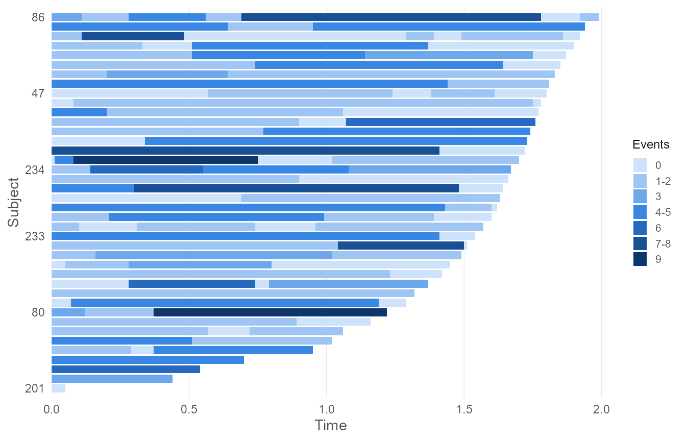
Two features of this plot affect the analysis. Alignment of examination times across subjects determines the pooled-grid size and the cost of fitting the rate model. The raggedness of the right edge shows how much of the baseline tail rests on a handful of subjects.

How long they take

Speed is worth measuring, and worth measuring on the question you actually ask of a fitted model. A point estimate on its own is rarely the end of an analysis.

The comparison below uses time-invariant covariates. That is not a simplification for convenience: PanelSurv(ID, time, count) has one row per examination and cannot express a covariate that changes during follow-up, so this is the only ground on which the two packages fit the same data. Counts are generated exactly, since with fixed covariates the increments are independent Poisson with mean .

sim_fixed <- function(n, beta = c(1, -1), tau = 2, exam_mean = 4) {
  Lambda <- function(t) 8 * log(1 + t)
  do.call(rbind, lapply(seq_len(n), function(i) {
    nexam <- max(1L, rpois(1, exam_mean))
    exams <- sort(unique(round(runif(nexam, 0, runif(1, 0.9 * tau, tau)), 2)))
    exams <- exams[exams > 0]
    x1 <- runif(1); x2 <- runif(1)
    mu <- diff(c(0, Lambda(exams))) * exp(beta[1] * x1 + beta[2] * x2)
    data.frame(id = i, time = exams, count = rpois(length(exams), mu),
               x1 = x1, x2 = x2)
  }))
}

d <- sim_fixed(200)

# pcdreg: the standard error comes back with the fit.
system.time({
  f <- pcdreg(pcd(id, time, count) ~ x1 + x2, data = d, model = "mean")
  sqrt(diag(vcov(f, "robust")))
})

# spef: a point estimate, then a standard error by resampling.
system.time(panelReg(PanelSurv(id, time, count) ~ x1 + x2, d,
                     method = "EE.HSWc", se = "NULL"))
system.time(panelReg(PanelSurv(id, time, count) ~ x1 + x2, d,
                     method = "EE.HSWc", se = "Bootstrap"))

Which standard errors are available

The route to a standard error differs by method, and this drives the timings more than the estimation does. For the Hu–Sun–Wei estimating equations, se = "Sandwich" and se = "Impute" both error, leaving the bootstrap:

spef method	se = "NULL"	"Sandwich"	"Impute"	"Bootstrap"
AEE	no SE	no SE	SE	SE
AEEX	no SE	SE	SE	SE
EE.HSWc	no SE	error	error	SE
EE.HSWm	no SE	error	error	SE
MPL	no SE	error	error	SE

pcdreg has no equivalent row. and are by-products of the last EM iteration, so vcov() is a pair of small matrix inversions on quantities the fit already computed.

Timings

Median of 3 replicates, in seconds.

bench <- data.frame(
  method = rep(c("pcdreg mean", "pcdreg rate", "spef AEE", "spef EE.HSWc",
                 "spef EE.HSWm", "spef MPL"), each = 4, times = 2),
  framing = rep(c("estimate + SE", "estimate only"), each = 24),
  n = rep(c(50, 100, 200, 400), times = 12),
  seconds = c(
    0.00, 0.00, 0.00, 0.00,   0.66, 1.83, 4.84, 7.23,
    0.89, 1.65, 3.17, 6.38,   0.15, 0.35, 0.79, 3.53,
    0.45, 0.89, 1.77, 5.23,   1.57, 2.27, 3.69, 4.98,
    0.00, 0.00, 0.00, 0.00,   0.66, 1.80, 4.89, 7.30,
    0.08, 0.11, 0.08, 0.11,   0.01, 0.03, 0.04, 0.14,
    0.01, 0.05, 0.08, 0.19,   0.04, 0.11, 0.12, 0.24
  )
)
knitr::kable(
  stats::reshape(bench, idvar = c("method", "framing"), timevar = "n",
                 direction = "wide"),
  col.names = c("method", "framing", "n = 50", "n = 100", "n = 200", "n = 400"),
  row.names = FALSE
)

method	framing	n = 50	n = 100	n = 200	n = 400
pcdreg mean	estimate + SE	0.00	0.00	0.00	0.00
pcdreg rate	estimate + SE	0.66	1.83	4.84	7.23
spef AEE	estimate + SE	0.89	1.65	3.17	6.38
spef EE.HSWc	estimate + SE	0.15	0.35	0.79	3.53
spef EE.HSWm	estimate + SE	0.45	0.89	1.77	5.23
spef MPL	estimate + SE	1.57	2.27	3.69	4.98
pcdreg mean	estimate only	0.00	0.00	0.00	0.00
pcdreg rate	estimate only	0.66	1.80	4.89	7.30
spef AEE	estimate only	0.08	0.11	0.08	0.11
spef EE.HSWc	estimate only	0.01	0.03	0.04	0.14
spef EE.HSWm	estimate only	0.01	0.05	0.08	0.19
spef MPL	estimate only	0.04	0.11	0.12	0.24

library(ggplot2)
#> Warning: package 'ggplot2' was built under R version 4.5.2
ggplot(bench, aes(n, seconds, colour = method)) +
  geom_line(linewidth = 0.6) +
  geom_point(size = 1.6) +
  facet_wrap(~ framing) +
  scale_colour_manual(values = c(
    "pcdreg mean"  = "#3987e5", "pcdreg rate"  = "#0d366b",
    "spef AEE"     = "#b0aca4", "spef EE.HSWc" = "#8a857c",
    "spef EE.HSWm" = "#645f57", "spef MPL"     = "#3f3b35")) +
  labs(x = "Subjects", y = "Median seconds", colour = NULL) +
  theme_minimal(base_size = 10) +
  theme(panel.grid.minor = element_blank())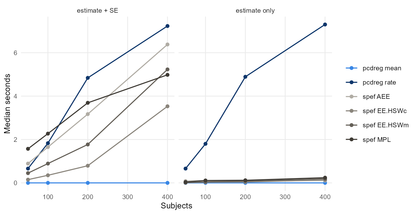

Read the two panels separately, because they reverse.

For a point estimate, spef is faster than the rate model and stays under a quarter of a second throughout. The rate model is doing nonparametric maximum likelihood by EM over a pooled grid, which is more work than solving an estimating equation, and it is the only method here that admits time-varying covariates at all.

For an estimate with a standard error, the ordering changes. pcdreg’s means model returns below timer resolution at every sample size, against 3.5 seconds for spef’s EE.HSWc, which is the same estimator reached by the same estimating equation. The difference is entirely the bootstrap. The rate model lands among the spef methods rather than behind them: 7.2 seconds at against 6.4 for AEE and 5.0 for MPL.

Why the rate model flattens

Its cost scales with , where is the number of distinct examination times pooled across subjects. Here was 119, 169, 195 and 198 as went 50, 100, 200, 400. Examination times rounded to two decimals on a bounded interval cannot keep producing new values, so saturates and the cost becomes roughly linear in rather than quadratic. Times carried at full numerical precision never tie, grows with , and the same fit becomes much more expensive. Rounding to the precision at which visits were actually scheduled is worth doing; see vignette("data-preparation").

Caveats

Run times for the rate model vary with the data, not just its size: three replicates at took 0.49, 0.66 and 6.59 seconds, since the number of EM iterations depends on the sample drawn. The medians above hide that spread.

MPL fits a monotone spline baseline and is solving a harder problem than the estimating equations, so its timing buys something the others do not provide.

Measured on one Windows 11 machine, R 4.5.1, spef 1.0.9, single threaded. Ratios between methods will travel better than the absolute numbers.

Which to use

If you need	Use
the rate model, or covariates that change between visits	pcdreg
standard errors that survive overdispersion	pcdreg
the mean model with the Hu–Sun–Wei estimating equation	either; pcdreg returns the standard error with the fit
many refits, as in a simulation or a bootstrap of your own	pcdreg(model = "mean")
informative observation or censoring times	spef (AEE, AEEX)
a monotone spline baseline mean	spef (MPLs, MLs)
an accelerated mean model, or the other mean-model estimators	spef
exactly observed event times	not panel count data; see reReg

pcdreg is deliberately narrow. It implements two models with covariance estimation worked out and tested. Use spef when it provides an estimator you need.

Reference

Sun, D., Guo, Y., Li, Y., Tu, W. and Sun, J. (2024). A robust approach for regression analysis of panel count data. Bernoulli 30(4), 3251–3275. doi:10.3150/23-BEJ1713