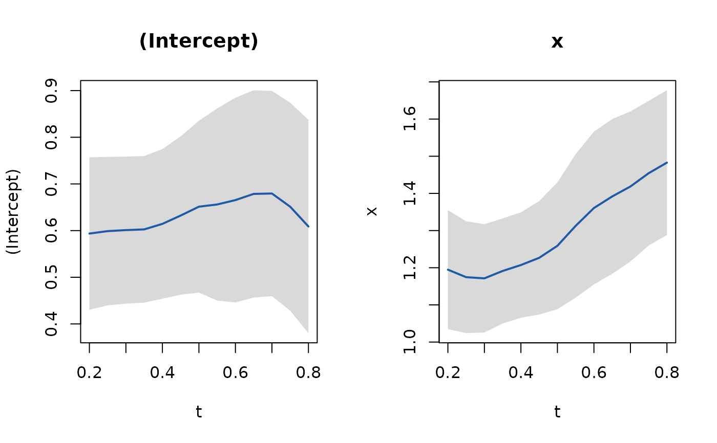
Plot estimated coefficient curves — plot.kee

Draws \(\hat\beta_j(t)\) against t with pointwise Wald bands, one panel per coefficient.

Usage

# S3 method for class 'kee_td'
plot(x, which = seq_len(ncol(x$coefficients)), level = 0.95, ...)

Arguments

x: A kee_td object from kee_async_td().
which: Integer or character vector selecting coefficients to draw. Defaults to all.
level: Confidence level for the pointwise bands.
...: Passed to graphics::plot().

Value

x, invisibly. Called for the plot.

Details

Each band covers its own target time. Reading them together as a region for the whole curve overstates the evidence. They also carry no correction for smoothing bias, so they cover \(E\hat\beta(t)\) instead of \(\beta(t)\): a large bandwidth flattens the curve without widening the band to say so.

Examples

set.seed(1)
d <- sim_async_data(n = 200, beta = function(tt) cbind(0.5, 1 + tt))
fit <- d$y |>
  kee_async_td(d$x, y ~ x,
    id = id, time = time,
    times = seq(0.2, 0.8, by = 0.05), h = 0.3
  )
plot(fit)