Getting Started with skmle

Overview

A longitudinal covariate is rarely measured at the time you need it. skmle handles that mismatch by weighting each observation according to how far its measurement time sits from the time being modelled, rather than carrying a value forward or smoothing the covariate and substituting it.

Two outcome types are covered.

Survival outcomes, where the covariate is observed sparsely and intermittently over follow-up:

1. skmle() for the general transformed hazards model.
2. kee_cox() for the proportional hazards estimating-equation approach.
3. kee_additive() for the additive hazards estimating-equation approach.

Asynchronous longitudinal outcomes, where the outcome is itself a sparsely observed process recorded on a time grid that does not line up with the covariate’s:

4. kee_async() for time-invariant coefficients.
5. kee_async_td() for a coefficient curve \(\beta(t)\).

This vignette walks through both: simulate data, fit a model, inspect the summary output, plot the estimated baseline component, select a bandwidth by cross-validation, then move to the asynchronous longitudinal setting.

Which function do I need?

Two questions.

First, what is the outcome? A time to an event (death, relapse, failure), possibly censored? Use the survival estimators; your data is one long table. Or a repeatedly measured quantity (a score, a lab value) recorded on its own schedule? Use the asynchronous estimators; your data is two tables.

Then:

Outcome	Situation	Function
Survival	Start here; Cox model	kee_cox()
Survival	Additive hazards instead	kee_additive()
Survival	Want the baseline hazard, or a model between the two	skmle()
Survival	Choose the bandwidth properly	skmle_cv()
Longitudinal	Start here; one constant effect	kee_async()
Longitudinal	Choose the bandwidth properly	kee_async_cv()
Longitudinal	The effect may change over time	kee_async_td()

Every fitting function picks a bandwidth for you if you do not supply one, and says in a message what it chose. That is enough for a first answer; the _cv() functions choose it from the data, which is what to report.

library(nloptr)
library(skmle)
library(survival)

Simulating some data

set.seed(123)

dat <- sim_skmle_data(
  n = 80,
  mu = function(tt) 8 * (0.75 + (0.5 - tt)^2),
  mu_bar = 8,
  alpha = function(tt) 0.5 * 0.75 + 0.75 * (tt * (1 - sin(2 * pi * (tt - 0.25)))),
  beta = c(1, -0.5),
  s = 0,
  cen = 0.7
)

head(dat)
#> # A tibble: 6 × 6
#>   id        X delta covariates[,1]  [,2] obs_times censoring
#>   <chr> <dbl> <lgl>          <dbl> <dbl>     <dbl>     <dbl>
#> 1 1     0.550 TRUE         0.419       1     0.129     0.930
#> 2 1     0.550 TRUE         0.593       1     0.217     0.930
#> 3 1     0.550 TRUE         0.593       1     0.247     0.930
#> 4 1     0.550 TRUE         0.412       1     0.433     0.930
#> 5 1     0.550 TRUE         0.933       1     0.798     0.930
#> 6 2     0.747 TRUE        -0.00422     1     0.288     0.865

The simulated data are stored in long format. Each row corresponds to one observed longitudinal measurement time for one subject.

The key columns are:

• id: subject identifier
• X: observed event or censoring time
• delta: event indicator
• covariates: observed covariate values at that visit time
• obs_times: longitudinal observation time

Fitting the general transformed hazards model

The covariates column returned by sim_skmle_data() is a matrix. You can either use it directly in the formula or split it into separate columns. Using the matrix directly is convenient for routine work.

fit_skmle <- skmle(
  Surv(X, delta) ~ covariates,
  data = dat,
  id = id,
  obs_times = obs_times,
  s = 0,
  h = 0.5,
  nknots = 3
)

fit_skmle
#> Call:
#> skmle(formula = Surv(X, delta) ~ covariates, data = dat, id = id, 
#>     obs_times = obs_times, s = 0, h = 0.5, nknots = 3)
#> 
#> Coefficients:
#> covariates1 covariates2 
#>   1.0297295  -0.4157912

The printed object gives the fitted coefficients. As in many R model objects, the formatted inferential output is produced by summary().

summary(fit_skmle)
#> Call:
#> skmle(formula = Surv(X, delta) ~ covariates, data = dat, id = id, 
#>     obs_times = obs_times, s = 0, h = 0.5, nknots = 3)
#> 
#>   n= 80
#> 
#>             Estimate Std. Error z value Pr(>|z|)  
#> covariates1  1.02973    0.41714  2.4686  0.01357 *
#> covariates2 -0.41579    0.28015 -1.4842  0.13776  
#> ---
#> Signif. codes:  0 '***' 0.001 '**' 0.01 '*' 0.05 '.' 0.1 ' ' 1
#> 
#> Log-likelihood: -0.1331

The summary table reports:

• coefficient estimates
• standard errors
• z statistics
• p-values

Plotting the baseline

plot(fit_skmle)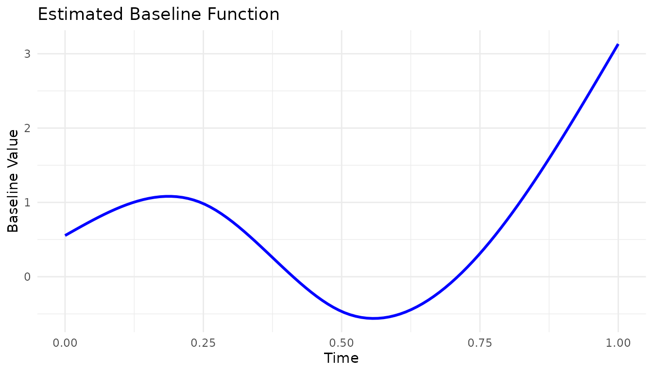

This plot visualizes the estimated nonparametric baseline component from the sieve fit.

The specialised estimating equations

When the model of interest matches one of the specialized settings, the package also provides dedicated estimating-equation estimators.

Cox-type

fit_kee_cox <- kee_cox(
  Surv(X, delta) ~ covariates,
  data = dat,
  id = id,
  obs_times = obs_times,
  h = 0.5
)

summary(fit_kee_cox)
#> Call:
#> kee_cox(formula = Surv(X, delta) ~ covariates, data = dat, id = id, 
#>     obs_times = obs_times, h = 0.5)
#> 
#> Cox-type proportional hazards, kernel estimating equation (half kernel)
#>   n= 80 subjects   bandwidth h = 0.5
#> 
#>             Estimate Std. Error z value Pr(>|z|)   
#> covariates1  1.02085    0.36037  2.8328 0.004615 **
#> covariates2 -0.36751    0.29950 -1.2271 0.219797   
#> ---
#> Signif. codes:  0 '***' 0.001 '**' 0.01 '*' 0.05 '.' 0.1 ' ' 1

Additive hazards

For the additive hazards estimator, simulate data under s = 1.

set.seed(456)

dat_add <- sim_skmle_data(
  n = 80,
  mu = function(tt) 8 * (0.75 + (0.5 - tt)^2),
  mu_bar = 8,
  alpha = function(tt) 0.75 + 0.75 * (tt * (1 - sin(2 * pi * (tt - 0.25)))),
  beta = c(1, -0.5),
  s = 1,
  cen = 0.7
)

fit_kee_add <- kee_additive(
  Surv(X, delta) ~ covariates,
  data = dat_add,
  id = id,
  obs_times = obs_times,
  h = 0.5
)

summary(fit_kee_add)
#> Call:
#> kee_additive(formula = Surv(X, delta) ~ covariates, data = dat_add, 
#>     id = id, obs_times = obs_times, h = 0.5)
#> 
#> Additive hazards, kernel estimating equation (half kernel)
#>   n= 80 subjects   bandwidth h = 0.5
#> 
#>             Estimate Std. Error z value Pr(>|z|)  
#> covariates1  0.94335    0.47788  1.9740  0.04838 *
#> covariates2 -0.41208    0.65185 -0.6322  0.52728  
#> ---
#> Signif. codes:  0 '***' 0.001 '**' 0.01 '*' 0.05 '.' 0.1 ' ' 1

Selecting a bandwidth

Bandwidth selection can be handled by skmle_cv().

set.seed(999)

cv_fit <- skmle_cv(
  Surv(X, delta) ~ covariates,
  data = dat,
  id = id,
  obs_times = obs_times,
  s = 0,
  K = 3,
  h_grid = c(0.3, 0.4, 0.5),
  nknots = 3,
  quiet = TRUE
)

cv_fit$h_cv
#> [1] 0.5
cv_fit$cv_results
#> # A tibble: 3 × 2
#>       h cvloss
#>   <dbl>  <dbl>
#> 1   0.3  0.758
#> 2   0.4  0.729
#> 3   0.5  0.699

The returned object contains:

• the selected bandwidth
• the refitted skmle model at that bandwidth
• the cross-validation loss table

You can then inspect the final refit in the usual way.

summary(cv_fit$fit)
#> Call:
#> skmle::skmle(formula = Surv(X, delta) ~ covariates, data = dat, 
#>     id = id, obs_times = obs_times, s = 0, nknots = 3, h = 0.5)
#> 
#>   n= 80
#> 
#>             Estimate Std. Error z value Pr(>|z|)  
#> covariates1  1.02973    0.41714  2.4686  0.01357 *
#> covariates2 -0.41579    0.28015 -1.4842  0.13776  
#> ---
#> Signif. codes:  0 '***' 0.001 '**' 0.01 '*' 0.05 '.' 0.1 ' ' 1
#> 
#> Log-likelihood: -0.1331

Half kernel or full kernel

Every estimator weights a covariate observation by how far it sits from the time being modelled. By default that window is one-sided: only observations strictly before the time contribute, which is the risk-set restriction of a hazard model. Set one_sided = FALSE to smooth the covariate path from both sides instead.

fit_full <- kee_cox(
  Surv(X, delta) ~ covariates,
  data = dat, id = id, obs_times = obs_times,
  h = 0.5, one_sided = FALSE
)
cbind(half = coef(fit_kee_cox), full = coef(fit_full))
#>                  half       full
#> covariates1  1.020846  0.8561813
#> covariates2 -0.367506 -0.3589201

The switch reaches the risk-set averages inside the C++ backend as well as the row weights, so the two halves of the estimator always use the same support. skmle_cv() takes it too, so the bandwidth is selected under the same kernel the final fit uses.

Asynchronous longitudinal data

The estimators above model a survival outcome. When the outcome is itself a sparsely observed longitudinal process, measured at times that do not line up with the covariate’s measurement times, use the kernel-weighted estimating equations of Cao, Zeng and Fine (2015). Nothing is carried forward and no pair is discarded: each (response, covariate) pair contributes in proportion to its time separation.

set.seed(202)
d <- sim_async_data(n = 300, beta = c(0.5, 1.5))
head(d$y, 3)
#> # A tibble: 3 × 3
#>      id  time     y
#>   <int> <dbl> <dbl>
#> 1     1 0.204 0.306
#> 2     1 0.330 0.430
#> 3     1 0.368 0.298
head(d$x, 3)
#> # A tibble: 3 × 3
#>      id   time      x
#>   <int>  <dbl>  <dbl>
#> 1     1 0.0763 -0.466
#> 2     1 0.198  -0.835
#> 3     1 0.219  -0.688

The two tables are deliberately separate. They sit on different grids, so no single data frame holds both without inventing rows. The formula spans both: its left-hand side is looked up in data_y, its right-hand side in data_x, and id and time name columns present in each.

fit_a <- kee_async(d$y, d$x,
  y ~ x,
  id = id, time = time, h = 0.25
)
summary(fit_a)
#> Call:
#> kee_async(data_y = d$y, data_x = d$x, formula = y ~ x, id = id, 
#>     time = time, h = 0.25)
#> 
#> Asynchronous longitudinal regression (identity link, full kernel)
#>   n= 300 subjects   bandwidth h = 0.25
#> 
#>             Estimate Std. Error z value  Pr(>|z|)    
#> (Intercept) 0.610058   0.065411  9.3266 < 2.2e-16 ***
#> x           1.336571   0.057907 23.0815 < 2.2e-16 ***
#> ---
#> Signif. codes:  0 '***' 0.001 '**' 0.01 '*' 0.05 '.' 0.1 ' ' 1
#> 
#> Optimization status: 0
confint(fit_a)
#>                 2.5 %    97.5 %
#> (Intercept) 0.4818555 0.7382607
#> x           1.2230761 1.4500656

The bandwidth is the one consequential choice. kee_async_cv() selects it by cross-validation over subjects, scoring each candidate by the kernel-weighted squared error on the held-out subjects:

cv <- kee_async_cv(d$y, d$x,
  y ~ x, id = id, time = time,
  h_grid = c(0.10, 0.15, 0.25, 0.40), K = 5, seed = 1, quiet = TRUE
)
#> Warning: the selected bandwidth is at an endpoint of 'h_grid'; widen the grid
#> to check that the minimum is interior
cv
#> Call:
#> kee_async_cv(data_y = d$y, data_x = d$x, formula = y ~ x, id = id, 
#>     time = time, h_grid = c(0.1, 0.15, 0.25, 0.4), K = 5, seed = 1, 
#>     quiet = TRUE)
#> 
#> 5-fold subject-level cross-validation
#> 
#> # A tibble: 4 × 3
#>       h cvloss nfold_used
#>   <dbl>  <dbl>      <dbl>
#> 1  0.1    1.09          5
#> 2  0.15   1.16          5
#> 3  0.25   1.27          5
#> 4  0.4    1.42          5
#> 
#> Selected h = 0.1
#> 
#> Coefficients at the refit:
#> (Intercept)           x 
#>   0.6264998   1.3661731

If the coefficients themselves vary with time, kee_async_td() estimates the curve \(\beta(t)\) pointwise. Both time arguments are smoothed there, so it converges at the bivariate rate \((n h_1 h_2)^{1/2}\) and the bands are wide.

set.seed(203)
dt <- sim_async_data(
  n = 500, beta = function(tt) cbind(0.5, 1 + tt),
  lambda_y = 8, lambda_x = 8,
  x_cov = function(s, t) exp(-4 * (s - t)^2)
)
fit_td <- kee_async_td(dt$y, dt$x,
  y ~ x, id = id, time = time,
  times = seq(0.2, 0.8, by = 0.05), h = 0.2
)
plot(fit_td)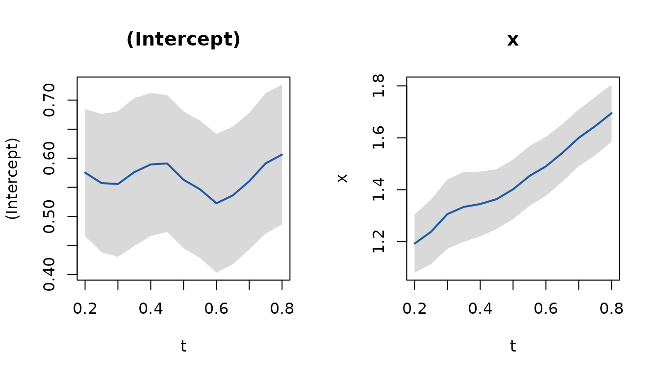

The asynchronous article covers this properly: why last-value-carried-forward and regression calibration fail here, how to read the bandwidth diagnostics, and what the half kernel changes.

A typical workflow

For routine use, the usual sequence is:

1. Prepare data in long format with one row per observation time.
2. Fit skmle() if you want the general transformed hazards model.
3. Use summary() and plot() to inspect the fitted model.
4. Use skmle_cv() if you want data-driven bandwidth selection.
5. Use kee_cox() or kee_additive() when the scientific model matches those specialized estimators.
6. Use kee_async() or kee_async_td() when the outcome is longitudinal rather than a survival time.

This gives a standard R model-fitting interface while keeping the core numerical work in the Rcpp backend.